import numpy as np
import pandas as pdPandas and Matplotlib
Feeding Pandas
Pandas
pandas is the Python library for working with tables of data. Where NumPy works with arrays of any dimension, pandas specialises in one and two dimensions:
- a
Seriesis one-dimensional: think of a single column - a
DataFrameis two-dimensional: a table, which is really a collection of columns
Pandas can be confusing for newcomers, because of a number of odd (historical) choices that were made along the way. Nearly all of them have to do with two things:
- the dtypes, in particular how missing data is handled
- the index
We will therefore start with Series objects. They are simpler than DataFrames, but they already have all of these problems. Once we understand those, we move on to DataFrames, and then we feed pandas some real data.
By convention, pandas is imported as pd:
A practical note before we start. When something goes wrong deep inside pandas, the traceback is very long, because it lists every function call inside pandas on the way to the error. In these notes I only want to show you the error message itself, so I switch IPython to minimal tracebacks. This is a so-called magic command, which only works in Jupyter and IPython, not in an ordinary script:
%xmode MinimalException reporting mode: MinimalIn your own notebook you will see the full traceback. Read it from the bottom up: the last line tells you what went wrong, and a little higher up you will find the line of your code that triggered it.
pandas 3
pandas 3.0 was released in January 2026, and it changed some long-standing behaviour. These notes use pandas 3. Most of the pandas code you will find online, and much of what AI assistants suggest, was written for pandas 2 or older, so where it matters I will point out what used to be different. Check which version you have:
pd.__version__'3.0.6'Series and their dtypes
Numbers
Just like a NumPy array, a Series has a dtype. It is derived from whatever you put in it:
my_series = pd.Series([1, 2, 3])
my_series
0 1
1 2
2 3
dtype: int64Notice the column of numbers on the left. That is the index, which will keep us busy for most of this lecture. For now, ignore it.
Sometimes it is better to be explicit about the dtype:
pd.Series([1, 2, 3], dtype="int32")0 1
1 2
2 3
dtype: int32Pandas uses NumPy as a backend: behind every numeric Series is a NumPy array, which you can get with .to_numpy():
pandas_series = pd.Series([1, 2, 3])
numpy_array = pandas_series.to_numpy()
numpy_array
array([1, 2, 3])In older versions of pandas, this was (usually!) a view on the same memory, so modifying the array would modify the Series behind your back. pandas 3 protects you from that: the array you get is read-only.
numpy_array[0] = 100ValueError: assignment destination is read-only
If you want an array you can modify, ask for a copy with .to_numpy(copy=True).
Here is another place where pandas 3 is stricter than NumPy. Remember how NumPy silently turned 100.7 into 100 when we stored it in an integer array? Pandas refuses:
s = pd.Series([1, 2, 3])
s[0] = 1.5TypeError: Invalid value '1.5' for dtype 'int64'
If you want floats, say so: s = s.astype("float64"). (Since pandas 2.1 this gave a warning, and before that, pandas silently converted the whole Series to floats for you.)
Object: the junk drawer
Like NumPy, pandas picks a dtype that can hold everything you give it. If there is no sensible choice, you get object, which means: a list of pointers to arbitrary Python objects.
pd.Series([1, 1.0])0 1.0
1 1.0
dtype: float64pd.Series([1, "a"])0 1
1 a
dtype: objectAn object Series is slow, takes a lot of memory, and anything goes inside of it. And since most operations preserve the dtype, an object column tends to infect everything it touches. Suppose you read some data, and somewhere in there is an empty string:
my_series = pd.Series([1, 2, 3, 4, ""])
my_series
0 1
1 2
2 3
3 4
4
dtype: objectTake the first three elements, which are all perfectly good integers. The dtype is still object:
my_series.head(3)0 1
1 2
2 3
dtype: objectAnd add an ordinary integer Series to it. Still object:
my_series.head(3) + pd.Series([1, 2, 3])0 2
1 4
2 6
dtype: objectEvery calculation that follows will be slow, and some will fail in confusing ways. The fix is to convert as early as possible, and to decide explicitly what should happen to the values that don’t fit:
pd.to_numeric(my_series, errors="coerce")0 1.0
1 2.0
2 3.0
3 4.0
4 NaN
dtype: float64
Tip
Always look at the dtypes of your data, very carefully. When you read data, be explicit about the types you expect and convert right away, rather than solving mysterious problems later on.
Missing data
Missing data is a nuisance for data analysis, and it is a nuisance for pandas as well.
Pandas interprets None as missing data. In a numeric Series, missing data is stored as the float NaN that we met in the previous lecture. And since NaN is a float, a Series of integers with one missing value becomes a Series of floats:
pd.Series([1.0, 2.0, None])0 1.0
1 2.0
2 NaN
dtype: float64pd.Series([1, 2, None])0 1.0
1 2.0
2 NaN
dtype: float64The problem is that integers have no special value that can mean “missing”. But even for floats the situation is not ideal: NaN can also be the legitimate result of a calculation (say, 0/0), and once it is in your data you can no longer tell the two apart. Pandas chose NaN for missing data long ago, mostly for simplicity and performance.
As an alternative, pandas offers nullable dtypes, which keep track of missing values separately and use a dedicated marker pd.NA. You recognise them by their capital letter:
pd.Series([1, None, 3], dtype="Int64")0 1
1 <NA>
2 3
dtype: Int64pd.Series([1.0, None, 3.0], dtype="Float64")0 1.0
1 <NA>
2 3.0
dtype: Float64.convert_dtypes() converts a Series (or a whole DataFrame) to these dtypes for you:
pd.Series([1, None, 3]).convert_dtypes()0 1
1 <NA>
2 3
dtype: Int64These dtypes have serious advantages, but they are still not the default, and you will see them much less often in practice.
An important difference with NumPy: pandas skips missing values in calculations by default.
s = pd.Series([1, 2, 3, None])
s.sum(), s.mean()
(np.float64(6.0), np.float64(2.0))np.array([1, 2, 3, np.nan]).sum()np.float64(nan)The methods .isna(), .notna(), .fillna(...) and .dropna() help you find, replace or remove missing values.
Strings
In pandas 3, a Series of strings gets a dedicated string dtype, simply called str:
pd.Series(["a", "b"])0 a
1 b
dtype: strIn pandas 2 and earlier, this would have been an object Series, so if you read older code (or older advice), object very often means “text”. The str dtype only accepts strings and missing values, and missing values are, once again, NaN:
pd.Series(["a", "b", None])0 a
1 b
2 NaN
dtype: strJust to keep things interesting, there is a second string dtype, "string", which predates pandas 3. It is one of the nullable dtypes, and uses pd.NA instead of NaN:
pd.Series(["a", "b", None], dtype="string")0 a
1 b
2 <NA>
dtype: stringFor everyday work the difference rarely matters, but be aware that both exist.
Dates and times
The same story once more. Pandas has its own dtype for timestamps, datetime64. When you create a Series from datetime objects, pandas converts them:
import datetime as dt

dates = pd.Series([dt.datetime(2026, 5, 7), dt.datetime(2026, 6, 7)])
dates
0 2026-05-07
1 2026-06-07
dtype: datetime64[us]The [us] means the timestamps are stored with microsecond resolution. (pandas 2 used nanoseconds by default, so you will often see datetime64[ns] too.) With the right dtype, the .dt accessor gives you all kinds of useful functionality:
dates.dt.year0 2026
1 2026
dtype: int32But if a single value does not fit, you are back to an object Series, and .dt no longer works:
messy_dates = pd.Series([dt.datetime(2026, 5, 7), dt.datetime(2026, 6, 7), "date unknown"])
messy_dates
0 2026-05-07 00:00:00
1 2026-06-07 00:00:00
2 date unknown
dtype: objectmessy_dates.dt.yearAttributeError: Can only use .dt accessor with datetimelike values
Use pd.to_datetime to convert explicitly, and decide what to do with the values that are not dates. With errors="coerce" they become NaT (“not a time”), the datetime version of NaN:
pd.to_datetime(messy_dates, errors="coerce").dt.year0 2026.0
1 2026.0
2 NaN
dtype: float64(Notice what the missing value did to the years: they are floats now. By now you can probably explain why.)
pd.to_datetime can also parse strings. But be very careful, because it guesses the format, and it guesses the American way:
pd.to_datetime(pd.Series(["01/02/2026", "03/04/2026"]))0 2026-01-02
1 2026-03-04
dtype: datetime64[us]If you meant the first of February, that is not what you got.
The PyArrow backend
Although pandas is built on NumPy, it can also store its columns as Apache Arrow arrays instead, if you have the pyarrow package installed. You ask for it through the dtype:
pd.Series([1, 2, None], dtype="int64[pyarrow]")Quoting the documentation, this gives you:
- more extensive data types compared to NumPy
- missing data support (NA) for all data types
- performant IO reader integration
- interoperability with other dataframe libraries based on the Apache Arrow specification (e.g. Polars)
In fact, the new str dtype quietly uses PyArrow behind the scenes if it is installed.
The index
Every Series has an index
Something else that leads to a lot of confusion is the index. A Series is not just a sequence of values: every value also has a label, its name if you like. The collection of all the labels is the index. By default the index is simply 0, 1, …, n-1, but in principle it can be anything:
pd.Series([0, 1, 2]) # default index0 0
1 1
2 2
dtype: int64pd.Series([0, 1, 2], index=[10, 20, 30]) # custom index10 0
20 1
30 2
dtype: int64pd.Series([0, 1, 2], index=["a", "b", "c"]) # string indexa 0
b 1
c 2
dtype: int64pd.Series([0, 1, 2], index=[("a", 1), ("a", 2), ("b", 1)]) # tuple index(a, 1) 0
(a, 2) 1
(b, 1) 2
dtype: int64Label or position?
Now here is the catch. The syntax s[key] does not select the element at position key, but the element with label key:
s = pd.Series([10, 11, 12, 13], index=[10, 20, 30, 40])
s[10]np.int64(10)s[0]KeyError: 0
So far, so good, you might say: [] uses labels. Except when it doesn’t. If you put a slice in the brackets, it suddenly works by position:
s[1:]20 11
30 12
40 13
dtype: int64s[1]KeyError: 1
s[1:] gives everything from position 1 onwards, but s[1] looks for the label 1. This is exactly the kind of thing that makes pandas code hard to read: you can’t tell what [] does without knowing what the index looks like at that moment.
What makes this especially treacherous is that selections keep their index. Start from the default index and take a slice:
s1 = pd.Series([10, 11, 12, 13])
s2 = s1[1:]
s2
1 11
2 12
3 13
dtype: int64s2 has no label 0, so s2[0] is a KeyError, even though s2 clearly has a first element.
at, iat, loc and iloc
The solution is to say explicitly what you mean. Pandas has four indexers for this:
| by label | by position | |
|---|---|---|
| a single element | .at[...] |
.iat[...] |
| a selection | .loc[...] |
.iloc[...] |
s2.at[1], s2.iat[0](np.int64(11), np.int64(11)).loc and .iloc accept slices, lists and more:
s = pd.Series([1, 2, 3, 4], index=["a", "b", "c", "d"])
s.loc["b":"c"]
b 2
c 3
dtype: int64s.iloc[1:2]b 2
dtype: int64Note that a slice in .loc includes the end label, while a slice in .iloc excludes the end position, just like Python does for lists. That is not as crazy as it seems: with labels, there is no way to know what the label “just after "c"” would be.
If you give .loc a single label, you get a single value, like .at. Give it a list with one label, and you get a Series:
s.loc["b"]np.int64(2)s.loc[["b"]]b 2
dtype: int64Finally, and most usefully, you can give .loc a Series of booleans. You get back the elements where it is True, just like a boolean mask in NumPy:
s = pd.Series([11, 12, 13, 14], index=["a", "b", "c", "d"])
selection = s % 2 == 0
selection
a False
b True
c False
d True
dtype: bools.loc[selection]b 12
d 14
dtype: int64Notice that selection is itself a Series, with the same index as s. Keep that in mind, it will matter in a moment.
Tip
To beginners with pandas I strongly recommend using .at, .iat, .loc and .iloc explicitly, as much as possible, and avoiding the plain s[...] until you are 100% comfortable with the index. Remember the Zen of Python: explicit is better than implicit. It will save you from strange errors when you accidentally get a single element where you expected a Series, or the other way around.
The index is not necessarily unique
Very, very confusing: the index does not have to be unique. So even .at can return a Series instead of a single value:
s = pd.Series([1, 2, 3], index=["a", "b", "a"])
s.at["a"]
a 1
a 3
dtype: int64You may think you would never create such an index. But perfectly ordinary operations do it for you. For instance, gluing two Series together with pd.concat keeps both indexes:
s1 = pd.Series([1, 2, 3])
s2 = pd.Series([10, 20, 30])
combined = pd.concat([s1, s2])
combined
0 1
1 2
2 3
0 10
1 20
2 30
dtype: int64combined.loc[1]1 2
1 20
dtype: int64There is always a solution, but you will only go looking for it if you already know the problem exists:
pd.concat([s1, s2], ignore_index=True)0 1
1 2
2 3
3 10
4 20
5 30
dtype: int64You can always check with s.index.is_unique.
What the index does: alignment
So far the index might seem like a nuisance that pandas makes you work around. Here is the reason it exists. Whenever you combine two Series, pandas matches up the elements by their label, not by their position. This is called alignment:
a = pd.Series([1, 2, 3], index=["a", "b", "c"])
b = pd.Series([10, 20, 30], index=["b", "c", "d"])
a + b
a NaN
b 12.0
c 23.0
d NaN
dtype: float64Labels that only appear on one side get NaN (and so our integers became floats, as we have come to expect). When the index means something, such as dates, product codes or names of people, this is wonderful: pandas makes sure you never add up values that don’t belong together, even if the data arrives in a different order.
But it bites you when you forget what the index is. Suppose you want the difference between consecutive values. In NumPy you would write x[1:] - x[:-1]. Try that in pandas:
values = pd.Series([10, 11, 13, 16])
values.iloc[1:] - values.iloc[:-1]
0 NaN
1 0.0
2 0.0
3 NaN
dtype: float64Each element is subtracted from itself, because the labels line up, and the ends become NaN. Pandas has a method for this particular calculation:
values.diff()0 NaN
1 1.0
2 2.0
3 3.0
dtype: float64And if you really want to work by position and ignore the labels, you can drop down to NumPy:
values.iloc[1:].to_numpy() - values.iloc[:-1].to_numpy()array([1, 2, 3])
When in doubt, look at the index
Most “pandas is giving me nonsense” moments are index problems. Whenever a result surprises you, print the index of everything involved. The tools to take control of it are reset_index(), set_index(...), ignore_index=True, and .to_numpy() when you deliberately want to throw the labels away.
Accessors and other useful methods
The dtype and the index aside, working with a Series is fairly intuitive. A few useful methods:
s = pd.Series([1, 2, 3])
s.astype("float64")
0 1.0
1 2.0
2 3.0
dtype: float64s.max(), s.min(), s.mean()(np.int64(3), np.int64(1), np.float64(2.0))s.describe()count 3.0
mean 2.0
std 1.0
min 1.0
25% 1.5
50% 2.0
75% 2.5
max 3.0
dtype: float64Some functionality is tucked away behind accessors, which only work for the right dtype. We already saw .dt for dates. The .str accessor treats every element as a string:
text = pd.Series(["xyz", "uvw", "abc"])
text.str[0]
0 x
1 u
2 a
dtype: strtext.str.startswith("x")0 True
1 False
2 False
dtype: boolIt has most of the methods of Python’s str, and a few extra. For instance .str.split can give you a DataFrame straight away, and .str.extract takes a regular expression (as in the standard libraries) and returns its groups:
codes = pd.Series(["ab:cd", "uv:xy", "no colon"])
codes.str.split(":", expand=True)| 0 | 1 | |
|---|---|---|
| 0 | ab | cd |
| 1 | uv | xy |
| 2 | no colon | NaN |
codes.str.extract(r"^(\w+):")| 0 | |
|---|---|
| 0 | ab |
| 1 | uv |
| 2 | NaN |
The .dt accessor has many more tricks:
moments = pd.to_datetime(pd.Series(["2026-10-24 00:00", "2026-10-25 01:00"]))
moments.dt.hour, moments.dt.day_name()
(0 0
1 1
dtype: int32,
0 Saturday
1 Sunday
dtype: str)
Note
There is also .apply(some_function), which calls an ordinary Python function on every element. It always works, but it is a Python loop in disguise, so it is slow. Look for a vectorised method or an accessor first, and use .apply as a last resort.
DataFrames
Creating DataFrames
A DataFrame is a table, and it is not much more than a collection of columns that share an index. Every column is a Series, so every column has a dtype, but rows do not.
The most common ways to create one by hand:
- from a dict of columns
- from a list of rows, plus the names of the columns
- from a list of records (dicts)
df = pd.DataFrame({
    "a": [10, 20, 30],
    "b": [100, 200, 300],
    "c": [7, 11, 13],
})
df| a | b | c | |
|---|---|---|---|
| 0 | 10 | 100 | 7 |
| 1 | 20 | 200 | 11 |
| 2 | 30 | 300 | 13 |
df = pd.DataFrame(
    [
        [10, 100, 7],
        [20, 200, 11],
        [30, 300, 13],
    ],
    columns=["a", "b", "c"],
    index=[10, 20, 30],
)
df| a | b | c | |
|---|---|---|---|
| 10 | 10 | 100 | 7 |
| 20 | 20 | 200 | 11 |
| 30 | 30 | 300 | 13 |
records = [
    {"a": 10, "b": 100, "c": 7},
    {"a": 20, "b": 200, "c": 11},
    {"a": 30, "b": 300, "c": 13},
]
pd.DataFrame(records)| a | b | c | |
|---|---|---|---|
| 0 | 10 | 100 | 7 |
| 1 | 20 | 200 | 11 |
| 2 | 30 | 300 | 13 |
A DataFrame has two indexes: df.index labels the rows, and df.columns labels the columns.
df.index, df.columns(Index([10, 20, 30], dtype='int64'), Index(['a', 'b', 'c'], dtype='str'))In practice, you will rarely type your data in by hand. Usually you read it from a file or a database: pd.read_csv, pd.read_excel, pd.read_json, pd.read_parquet, pd.read_sql, … And there is a matching df.to_csv, df.to_excel, … for every one of them. We already used to_csv in the lecture on files.
Selecting data
To select data in a DataFrame you use the same four indexers as for a Series, but now with two arguments: first the rows, then the columns.
df.at[row, column]df.iat[row_position, column_position]df.loc[rows, columns]df.iloc[row_positions, column_positions]
df = pd.DataFrame(
    [[1, "a", 3.14], [2, "b", 6.28], [3, "c", 9.42]],
    columns=["ix", "code", "value"],
)
df| ix | code | value | |
|---|---|---|---|
| 0 | 1 | a | 3.14 |
| 1 | 2 | b | 6.28 |
| 2 | 3 | c | 9.42 |
df.at[1, "code"], df.iat[1, 1]('b', 'b')df.loc[0:1, ["code", "value"]]| code | value | |
|---|---|---|
| 0 | a | 3.14 |
| 1 | b | 6.28 |
df.loc[df.value > 5, "code"]1 b
2 c
Name: code, dtype: strA single row comes out as a Series, whose index is the column names. Since a row can mix different types, its dtype is often object:
df.loc[0]ix 1
code a
value 3.14
Name: 0, dtype: objectFor columns there is a shortcut. df["code"] is the same as df.loc[:, "code"] and gives you a Series, while df[["code"]] gives you a DataFrame with one column. There is even df.code, which is very convenient but only works to read a column.
df["code"]0 a
1    b
2    c
Name: code, dtype: strTo create a new column, use the [] syntax:
df["new_column"] = df["value"] + df["ix"]
df| ix | code | value | new_column | |
|---|---|---|---|---|
| 0 | 1 | a | 3.14 | 4.14 |
| 1 | 2 | b | 6.28 | 8.28 |
| 2 | 3 | c | 9.42 | 12.42 |
If you try to do that with attribute syntax, pandas creates an ordinary Python attribute on the object, which is not a column at all. At least it warns you:
df.another_column = df["value"] * 2
df.columns
/tmp/ipykernel_12476/1268718135.py:1: UserWarning: Pandas doesn't allow columns to be created via a new attribute name - see https://pandas.pydata.org/pandas-docs/stable/indexing.html#attribute-access
df.another_column = df["value"] * 2Index(['ix', 'code', 'value', 'new_column'], dtype='str')Also be careful with columns that happen to have the same name as a method. Here df.max is the method, not the column:
df = pd.DataFrame([[1, "a", 3.14], [2, "b", 6.28]], columns=["ix", "code", "max"])
df.max
<bound method DataFrame.max of ix code max
0 1 a 3.14
1 2 b 6.28>df["max"]0 3.14
1 6.28
Name: max, dtype: float64
Tip
Use .at, .iat, .loc and .iloc as much as possible while you are learning pandas. When you are completely comfortable with the index, you can move to df[...] and df.column where they make your code shorter.
Sorting: an alignment trap
Here is the alignment trap in its most common form. You want to add a sorted version of a column to your DataFrame:
scores = pd.DataFrame({"name": ["jan", "piet", "joris"], "score": [30, 10, 20]})
scores["score_sorted"] = scores["score"].sort_values()
scores| name | score | score_sorted | |
|---|---|---|---|
| 0 | jan | 30 | 30 |
| 1 | piet | 10 | 10 |
| 2 | joris | 20 | 20 |
Nothing happened! Sorting a Series keeps each value together with its label. When you assign it as a column, pandas aligns it on the labels, which puts every value right back where it came from. If you want to sort, sort the whole table, so the rows stay together:
scores.sort_values("score")| name | score | score_sorted | |
|---|---|---|---|
| 1 | piet | 10 | 10 |
| 2 | joris | 20 | 20 |
| 0 | jan | 30 | 30 |
Note how the index now reads 1, 2, 0. If you want a fresh 0, 1, 2 you can add .reset_index(drop=True).
Modifying data: Copy-on-Write
Changing values in a DataFrame has historically been one of the most confusing parts of pandas. In pandas 3 the rule is simple, and it is called Copy-on-Write: every selection behaves as a copy. If you want to change df, change df itself, with .loc or .iloc:
df = pd.DataFrame({"a": [1, 2, 3], "b": [10, 20, 30]})
df.loc[df["a"] > 1, "b"] = 0
df| a | b | |
|---|---|---|
| 0 | 1 | 10 |
| 1 | 2 | 0 |
| 2 | 3 | 0 |
What does not work is chained assignment: two pairs of brackets in a row, where the first selects and the second assigns. The assignment goes to a temporary copy, and pandas tells you so:
df = pd.DataFrame({"a": [1, 2, 3], "b": [10, 20, 30]})
df[df["a"] > 1]["b"] = 0
df
/tmp/ipykernel_12476/4280215371.py:2: ChainedAssignmentError: A value is being set on a copy of a DataFrame or Series through chained assignment.
Such chained assignment never works to update the original DataFrame or Series, because the intermediate object on which we are setting values always behaves as a copy (due to Copy-on-Write).
Try using '.loc[row_indexer, col_indexer] = value' instead, to perform the assignment in a single step.
See the documentation for a more detailed explanation: https://pandas.pydata.org/pandas-docs/stable/user_guide/copy_on_write.html#chained-assignment
df[df["a"] > 1]["b"] = 0| a | b | |
|---|---|---|
| 0 | 1 | 10 |
| 1 | 2 | 20 |
| 2 | 3 | 30 |
And if you store a selection in a variable and modify that, only the selection changes:
df = pd.DataFrame({"a": [1, 2, 3], "b": [10, 20, 30]})
subset = df.loc[df["a"] > 1]
subset["b"] = 0
df| a | b | |
|---|---|---|
| 0 | 1 | 10 |
| 1 | 2 | 20 |
| 2 | 3 | 30 |
Note
In pandas 2 and earlier, the answer to “does changing this selection change the original?” was: it depends on whether pandas happened to make a view or a copy internally. The infamous SettingWithCopyWarning tried to warn you about this, and confused generations of data scientists. If you see it mentioned online, you now know where it came from. The Copy-on-Write guide explains the details.
Feeding pandas: a showcase
Time for some real data. We will use the Pokémon dataset that we already met in the first lecture, and work through the pandas functionality you will use most often.
Reading and inspecting
read_csv can read straight from a URL:
POKEMON_URL = "https://raw.githubusercontent.com/lgreski/pokemonData/master/Pokemon.csv"

df = pd.read_csv(POKEMON_URL)
df.dtypes
ID int64
Name str
Form str
Type1 str
Type2 str
Total int64
HP int64
Attack int64
Defense int64
Sp. Atk int64
Sp. Def int64
Speed int64
Generation int64
dtype: objectThe very first thing to do with any new dataset: look at the dtypes. Here they look reasonable. Next, look at some actual rows, at the start, at the end, and at random:
df.head(4)| ID | Name | Form | Type1 | Type2 | Total | HP | Attack | Defense | Sp. Atk | Sp. Def | Speed | Generation | |
|---|---|---|---|---|---|---|---|---|---|---|---|---|---|
| 0 | 1 | Bulbasaur | Grass | Poison | 318 | 45 | 49 | 49 | 65 | 65 | 45 | 1 | |
| 1 | 2 | Ivysaur | Grass | Poison | 405 | 60 | 62 | 63 | 80 | 80 | 60 | 1 | |
| 2 | 3 | Venusaur | Grass | Poison | 525 | 80 | 82 | 83 | 100 | 100 | 80 | 1 | |
| 3 | 4 | Charmander | Fire | 309 | 39 | 52 | 43 | 60 | 50 | 65 | 1 |
df.tail(4)| ID | Name | Form | Type1 | Type2 | Total | HP | Attack | Defense | Sp. Atk | Sp. Def | Speed | Generation | |
|---|---|---|---|---|---|---|---|---|---|---|---|---|---|
| 1211 | 1024 | Terapagos | Normal Form | Normal | 450 | 90 | 65 | 85 | 65 | 85 | 60 | 9 | |
| 1212 | 1024 | Terapagos | Terastal Form | Normal | 600 | 95 | 95 | 110 | 105 | 110 | 85 | 9 | |
| 1213 | 1024 | Terapagos | Stellar Form | Normal | 700 | 160 | 105 | 110 | 130 | 110 | 85 | 9 | |
| 1214 | 1025 | Pecharunt | Poison | Ghost | 600 | 88 | 88 | 160 | 88 | 88 | 88 | 9 |
df.sample(3, random_state=1) # random_state makes the "random" choice reproducible| ID | Name | Form | Type1 | Type2 | Total | HP | Attack | Defense | Sp. Atk | Sp. Def | Speed | Generation | |
|---|---|---|---|---|---|---|---|---|---|---|---|---|---|
| 838 | 731 | Pikipek | Normal | Flying | 265 | 35 | 75 | 30 | 30 | 30 | 65 | 7 | |
| 776 | 700 | Sylveon | Fairy | 525 | 95 | 65 | 65 | 110 | 130 | 60 | 6 | ||
| 341 | 342 | Crawdaunt | Water | Dark | 468 | 63 | 120 | 85 | 90 | 55 | 55 | 3 |
The column names contain spaces and dots, which is inconvenient. It is best to fix that immediately after reading the data. The .str accessor works on the column index too:
df.columns = df.columns.str.replace(".", "").str.replace(" ", "").str.lower()
df.columns
Index(['id', 'name', 'form', 'type1', 'type2', 'total', 'hp', 'attack',
'defense', 'spatk', 'spdef', 'speed', 'generation'],
dtype='str')Missing data in disguise
Are there any missing values?
df.isna().sum()id 0
name 0
form 0
type1 0
type2 0
total 0
hp 0
attack 0
defense 0
spatk 0
spdef 0
speed 0
generation 0
dtype: int64None at all, apparently. But plenty of Pokémon only have one type. What is in type2 for them?
df["type2"].value_counts().head(3)type2
546
Flying 122
Psychic 52
Name: count, dtype: int64The most common “type” is a single space! Whoever made this file encoded missing values as " ", and pandas has no way of knowing that this means “missing”. This is extremely common in real data: look out for empty strings, "-", "N/A", -1, 999, …
The best place to fix this is when reading the data. Let’s put the loading and cleaning in a function, so that we have one place where it happens:
def load_pokemon():
    df = pd.read_csv(POKEMON_URL, na_values=" ")
    df.columns = df.columns.str.replace(".", "").str.replace(" ", "").str.lower()
    return df

df = load_pokemon()
df.info()
<class 'pandas.DataFrame'>
RangeIndex: 1215 entries, 0 to 1214
Data columns (total 13 columns):
# Column Non-Null Count Dtype
--- ------ -------------- -----
0 id 1215 non-null int64
1 name 1215 non-null str
2 form 230 non-null str
3 type1 1215 non-null str
4 type2 669 non-null str
5 total 1215 non-null int64
6 hp 1215 non-null int64
7 attack 1215 non-null int64
8 defense 1215 non-null int64
9 spatk 1215 non-null int64
10 spdef 1215 non-null int64
11 speed 1215 non-null int64
12 generation 1215 non-null int64
dtypes: int64(9), str(4)
memory usage: 123.5 KBdf.info() gives you the dtypes, the number of non-missing values per column, and the memory use, all in one go. Now we can see that most Pokémon have no form and nearly half have no type2.
Is the data what you think it is?
The column total is supposed to be the sum of the six stats from hp up to and including speed. With .loc we can select that range of columns (remember, .loc slices include the end), and with axis=1 we sum each row, just like in NumPy:
df.loc[:, "hp":"speed"].head(3)| hp | attack | defense | spatk | spdef | speed | |
|---|---|---|---|---|---|---|
| 0 | 45 | 49 | 49 | 65 | 65 | 45 |
| 1 | 60 | 62 | 63 | 80 | 80 | 60 |
| 2 | 80 | 82 | 83 | 100 | 100 | 80 |
(df.loc[:, "hp":"speed"].sum(axis=1) == df["total"]).all()np.True_Checks like this are cheap, and they regularly catch problems with your data, or with your understanding of it.
Selecting rows
Boolean selections work just like in NumPy, including the &, |, ~ and the parentheses:
df.loc[(df["hp"] == 80) & (df["spatk"] == 100), ["name", "type1", "hp", "spatk"]]| name | type1 | hp | spatk | |
|---|---|---|---|---|
| 2 | Venusaur | Grass | 80 | 100 |
| 70 | Victreebel | Grass | 80 | 100 |
| 380 | Regice | Ice | 80 | 100 |
| 635 | Accelgor | Bug | 80 | 100 |
| 1059 | Regieleki | Electric | 80 | 100 |
row_selection = (df["type1"] == "Fire") | (df["type2"] == "Fire")
column_selection = ["name", "type1", "type2", "generation"]
df.loc[row_selection, column_selection].head(5)| name | type1 | type2 | generation | |
|---|---|---|---|---|
| 3 | Charmander | Fire | NaN | 1 |
| 4 | Charmeleon | Fire | NaN | 1 |
| 5 | Charizard | Fire | Flying | 1 |
| 36 | Vulpix | Fire | NaN | 1 |
| 37 | Ninetales | Fire | NaN | 1 |
.isin tests membership in a list:
df.loc[df["hp"].isin([99, 101]), ["name", "hp"]]| name | hp | |
|---|---|---|
| 359 | Tropius | 99 |
| 759 | Aromatisse | 101 |
| 1193 | Walking Wake | 99 |
Alternatively, .query lets you write the condition as a string, which some people find more readable:
df.query("hp == 80 and spatk == 100")[["name", "hp", "spatk"]]| name | hp | spatk | |
|---|---|---|---|
| 2 | Venusaur | 80 | 100 |
| 70 | Victreebel | 80 | 100 |
| 380 | Regice | 80 | 100 |
| 635 | Accelgor | 80 | 100 |
| 1059 | Regieleki | 80 | 100 |
df.query('name.str.startswith("C")').head(3)| id | name | form | type1 | type2 | total | hp | attack | defense | spatk | spdef | speed | generation | |
|---|---|---|---|---|---|---|---|---|---|---|---|---|---|
| 3 | 4 | Charmander | NaN | Fire | NaN | 309 | 39 | 52 | 43 | 60 | 50 | 65 | 1 |
| 4 | 5 | Charmeleon | NaN | Fire | NaN | 405 | 58 | 64 | 58 | 80 | 65 | 80 | 1 |
| 5 | 6 | Charizard | NaN | Fire | Flying | 534 | 78 | 84 | 78 | 109 | 85 | 100 | 1 |
Adding and removing columns
New columns are computed from existing ones. Since all the columns of a DataFrame share the same index, alignment does exactly what you would hope:
df["att_def"] = df["attack"] + df["defense"]
df[["name", "attack", "defense", "att_def"]].head(3)| name | attack | defense | att_def | |
|---|---|---|---|---|
| 0 | Bulbasaur | 49 | 49 | 98 |
| 1 | Ivysaur | 62 | 63 | 125 |
| 2 | Venusaur | 82 | 83 | 165 |
Most pandas methods do not modify the DataFrame, but return a new one. So you have to assign the result:
df = df.drop(columns="att_def")
df.columns
Index(['id', 'name', 'form', 'type1', 'type2', 'total', 'hp', 'attack',
'defense', 'spatk', 'spdef', 'speed', 'generation'],
dtype='str')(Many methods have an inplace=True argument as well. Don’t use it: it rarely saves anything, and it makes it harder to chain methods together, as we will do below.)
Counting things
Which values occur, how many different ones, and how often?
df["type1"].unique()<StringArray>
[ 'Grass', 'Fire', 'Water', 'Bug', 'Normal', 'Poison',
'Electric', 'Ground', 'Fairy', 'Fighting', 'Psychic', 'Rock',
'Ghost', 'Ice', 'Dragon', 'Dark', 'Steel', 'Flying']
Length: 18, dtype: strdf["type1"].nunique()18df["type1"].value_counts()type1
Water 150
Normal 134
Grass 113
Bug 91
Psychic 82
Fire 76
Electric 74
Rock 68
Dark 56
Fighting 50
Poison 49
Dragon 49
Ground 47
Ghost 47
Steel 45
Ice 43
Fairy 31
Flying 10
Name: count, dtype: int64Look carefully at that last result. It is a Series whose index consists of the types, so you can look up a type by label:
df["type1"].value_counts().at["Water"]np.int64(150)This is a general pattern: many pandas operations move some of your data into the index of the result. Keep track of it.
The index in practice
Our DataFrame has the default index 0, 1, 2, … Every Pokémon has a name, so wouldn’t the name be a much nicer index?
by_name = df.set_index("name")
by_name.loc["Bulbasaur", ["id", "form", "hp"]]
id 1
form NaN
hp 45
Name: Bulbasaur, dtype: objectThat looks great. Let’s look up Pikachu:
by_name.loc["Pikachu", ["id", "form", "hp"]]| id | form | hp | |
|---|---|---|---|
| name | |||
| Pikachu | 25 | NaN | 35 |
| Pikachu | 25 | Partner Pikachu | 45 |
There are two Pikachus, so we got a DataFrame instead of a Series. The very same line of code returns a different type depending on the data, which is a recipe for bugs that only show up for some inputs. The id is not unique either, because of the alternative forms. If an index is supposed to be unique, let pandas check it for you:
df.set_index("name", verify_integrity=True)ValueError: Index has duplicate keys: Index(['Nidoran', 'Castform', 'Deoxys', 'Burmy', 'Wormadam', 'Rotom', 'Giratina', 'Shaymin', 'Basculin', 'Darmanitan', ... 'Ursaluna', 'Oinkologne', 'Maushold', 'Squawkabilly', 'Palafin', 'Tatsugiri', 'Dudunsparce', 'Gimmighoul', 'Ogerpon', 'Terapagos'], dtype='str', name='name', length=153)
Grouping and aggregating
One of the most powerful features of pandas is groupby: split the data into groups, do a calculation per group, and combine the results. Recommended reading: the user guide on groupby.
groupby on its own gives you a “group by” object, you still have to do something with it:
grouped = df.groupby("type1")
grouped
<pandas.api.typing.DataFrameGroupBy object at 0x7917f85d9400>For instance, you can loop over it. Each time you get the name of the group, and the part of the DataFrame that belongs to it:
for type_name, group in grouped:
    print(type_name, group["hp"].sum())
    if type_name == "Electric":
        break
Bug 5169
Dark 4082
Dragon 4144
Electric 4724But mostly you apply an aggregation to it directly, which is faster and gives you a nice result:
grouped["hp"].sum().head()type1
Bug 5169
Dark 4082
Dragon 4144
Electric 4724
Fairy 2236
Name: hp, dtype: int64The column we grouped on has become the index of the result. You will often see these operations written as a method chain, one step per line, inside parentheses:
result = (
    df
    .loc[:, ["type1", "hp", "total"]]   # select columns
    .query('type1.str[0] < "G"')        # types starting with A to F
    .groupby("type1")                   # group by type
    .max()                              # maximum per group
)
result| hp | total | |
|---|---|---|
| type1 | ||
| Bug | 107 | 600 |
| Dark | 223 | 680 |
| Dragon | 216 | 780 |
| Electric | 125 | 670 |
| Fairy | 126 | 700 |
| Fighting | 154 | 700 |
| Fire | 115 | 680 |
| Flying | 98 | 580 |
If you want type1 back as an ordinary column, reset the index (or pass as_index=False to groupby):
result.reset_index()| type1 | hp | total | |
|---|---|---|---|
| 0 | Bug | 107 | 600 |
| 1 | Dark | 223 | 680 |
| 2 | Dragon | 216 | 780 |
| 3 | Electric | 125 | 670 |
| 4 | Fairy | 126 | 700 |
| 5 | Fighting | 154 | 700 |
| 6 | Fire | 115 | 680 |
| 7 | Flying | 98 | 580 |
To compute several things at once, with names of your own choosing, use .agg with named aggregations:
(
    df
    .groupby("generation")
    .agg(
        hp_max=("hp", "max"),
        hp_min=("hp", "min"),
        attack_mean=("attack", "mean"),
        count=("id", "count"),
    )
)| hp_max | hp_min | attack_mean | count | |
|---|---|---|---|---|
| generation | ||||
| 1 | 250 | 10 | 72.913907 | 151 |
| 2 | 255 | 20 | 68.260000 | 100 |
| 3 | 170 | 1 | 73.936170 | 141 |
| 4 | 150 | 20 | 79.127119 | 118 |
| 5 | 165 | 30 | 82.442424 | 165 |
| 6 | 126 | 38 | 94.923664 | 131 |
| 7 | 223 | 10 | 86.508197 | 122 |
| 8 | 255 | 25 | 86.197279 | 147 |
| 9 | 170 | 10 | 83.850000 | 140 |
Be careful with count: it counts the values that are not missing, per column. That is not necessarily the number of rows in the group, which is .size():
df.groupby("generation")[["id", "type2", "form"]].count().head(3)| id | type2 | form | |
|---|---|---|---|
| generation | |||
| 1 | 151 | 67 | 2 |
| 2 | 100 | 49 | 0 |
| 3 | 141 | 66 | 7 |
You can group by several columns at once. The result then has a MultiIndex: an index whose labels are tuples.
hp_per_gen_type = df.groupby(["generation", "type1"])["hp"].mean()
hp_per_gen_type.head()
generation type1
1 Bug 55.416667
Dragon 64.333333
Electric 54.444444
Fairy 82.500000
Fighting 63.571429
Name: hp, dtype: float64hp_per_gen_type.loc[(1, "Fire")]np.float64(63.833333333333336).unstack() moves the inner level of the index to the columns, which turns this into a table:
hp_per_gen_type.unstack().iloc[:4, :6]| type1 | Bug | Dark | Dragon | Electric | Fairy | Fighting |
|---|---|---|---|---|---|---|
| generation | ||||||
| 1 | 55.416667 | NaN | 64.333333 | 54.444444 | 82.5 | 63.571429 |
| 2 | 56.500000 | 66.0 | NaN | 61.666667 | 58.0 | 42.500000 |
| 3 | 49.833333 | 55.0 | 77.857143 | 57.500000 | NaN | 76.500000 |
| 4 | 55.833333 | 80.0 | 78.000000 | 57.500000 | 85.0 | 55.000000 |
An aggregation gives you one result per group. Sometimes you want one result per row instead, for instance: how much more HP does each Pokémon have than the average of its type? That is what .transform is for. Its result has the same index as df, so alignment lets you use it directly in a calculation:
df["hp_vs_type"] = df["hp"] - df.groupby("type1")["hp"].transform("mean")
df[["name", "type1", "hp", "hp_vs_type"]].head()| name | type1 | hp | hp_vs_type | |
|---|---|---|---|---|
| 0 | Bulbasaur | Grass | 45 | -22.318584 |
| 1 | Ivysaur | Grass | 60 | -7.318584 |
| 2 | Venusaur | Grass | 80 | 12.681416 |
| 3 | Charmander | Fire | 39 | -31.763158 |
| 4 | Charmeleon | Fire | 58 | -12.763158 |
A last common question: the top 2 Pokémon (by total) of every generation. Sort first, then take the first two rows of every group:
(
    df
    .sort_values("total", ascending=False)
    .groupby("generation")
    .head(2)
    .sort_values("generation")
    .loc[:, ["name", "form", "generation", "total"]]
)| name | form | generation | total | |
|---|---|---|---|---|
| 149 | Mewtwo | NaN | 1 | 680 |
| 148 | Dragonite | NaN | 1 | 600 |
| 248 | Lugia | NaN | 2 | 680 |
| 249 | Ho-oh | NaN | 2 | 680 |
| 288 | Slaking | NaN | 3 | 670 |
| 386 | Rayquaza | NaN | 3 | 680 |
| 498 | Palkia | NaN | 4 | 680 |
| 509 | Arceus | NaN | 4 | 720 |
| 668 | Kyurem | White Kyurem | 5 | 700 |
| 669 | Kyurem | Black Kyurem | 5 | 700 |
| 689 | Mewtwo | Mega Mewtwo Y | 6 | 780 |
| 688 | Mewtwo | Mega Mewtwo X | 6 | 780 |
| 828 | Zygarde | Complete Forme | 7 | 708 |
| 918 | Necrozma | Ultra Necrozma | 7 | 754 |
| 1052 | Zamazenta | Crowned Shield | 8 | 700 |
| 1054 | Eternatus | Eternamax | 8 | 1125 |
| 1213 | Terapagos | Stellar Form | 9 | 700 |
| 1192 | Miraidon | NaN | 9 | 670 |
Note
For anything that doesn’t fit in the patterns above, there is groupby(...).apply(function), which calls your function once for every group with that group’s DataFrame. It is the most flexible option, and the slowest. Note that in pandas 3 the function no longer gets to see the columns you grouped by.
Combining data: concat, join, merge
There are three ways to combine DataFrames. Recommended reading: the user guide on merging.
pd.concat glues DataFrames together, by default below each other. The columns are matched by name, and ignore_index=True gives us a fresh index:
first = df.head(3).loc[:, ["id", "hp", "generation"]]
last = df.tail(3).loc[:, ["id", "total", "generation"]]
pd.concat([first, last], ignore_index=True)| id | hp | generation | total | |
|---|---|---|---|---|
| 0 | 1 | 45.0 | 1 | NaN |
| 1 | 2 | 60.0 | 1 | NaN |
| 2 | 3 | 80.0 | 1 | NaN |
| 3 | 1024 | NaN | 9 | 600.0 |
| 4 | 1024 | NaN | 9 | 700.0 |
| 5 | 1025 | NaN | 9 | 600.0 |
With axis=1, concat puts them next to each other, and matches the rows by their index:
left = df.loc[[0, 1, 2], ["id", "name", "total"]]
right = df.loc[[0, 1, 3], ["id", "name", "hp"]]
pd.concat([left, right], axis=1)| id | name | total | id | name | hp | |
|---|---|---|---|---|---|---|
| 0 | 1.0 | Bulbasaur | 318.0 | 1.0 | Bulbasaur | 45.0 |
| 1 | 2.0 | Ivysaur | 405.0 | 2.0 | Ivysaur | 60.0 |
| 2 | 3.0 | Venusaur | 525.0 | NaN | NaN | NaN |
| 3 | NaN | NaN | NaN | 4.0 | Charmander | 39.0 |
.join also combines on the index, but adds a suffix to make the column names unique, which is a lot better. With how= you choose which rows to keep:
left.join(right, lsuffix="_left", rsuffix="_right")| id_left | name_left | total | id_right | name_right | hp | |
|---|---|---|---|---|---|---|
| 0 | 1 | Bulbasaur | 318 | 1.0 | Bulbasaur | 45.0 |
| 1 | 2 | Ivysaur | 405 | 2.0 | Ivysaur | 60.0 |
| 2 | 3 | Venusaur | 525 | NaN | NaN | NaN |
left.join(right, lsuffix="_left", rsuffix="_right", how="inner")| id_left | name_left | total | id_right | name_right | hp | |
|---|---|---|---|---|---|---|
| 0 | 1 | Bulbasaur | 318 | 1 | Bulbasaur | 45 |
| 1 | 2 | Ivysaur | 405 | 2 | Ivysaur | 60 |
Notice what happened to the dtypes along the way: id, total and hp turned into floats wherever a missing value appeared. Missing data strikes again.
.merge is the most general one. It does not look at the index, but at the columns you specify, like a JOIN in SQL:
ages = pd.DataFrame([["jan", 35], ["piet", 30], ["joris", 40]], columns=["name", "age"])
cities = pd.DataFrame(
    [["jan", "Gent"], ["piet", "Leuven"], ["korneel", "Brugge"]],
    columns=["name", "city"],
)
ages.merge(cities, on="name")| name | age | city | |
|---|---|---|---|
| 0 | jan | 35 | Gent |
| 1 | piet | 30 | Leuven |
The default is an inner merge: only names that occur on both sides survive. The alternatives are how="left", "right" and "outer". With indicator=True you can see where every row came from:
ages.merge(cities, on="name", how="outer", indicator=True)| name | age | city | _merge | |
|---|---|---|---|---|
| 0 | jan | 35.0 | Gent | both |
| 1 | joris | 40.0 | NaN | left_only |
| 2 | korneel | NaN | Brugge | right_only |
| 3 | piet | 30.0 | Leuven | both |
A classic mistake is to merge on a column that you think is unique, but isn’t. Every match is then repeated, and your data silently grows. If you know what the relationship should be, tell pandas with validate=, and it will check:
cities_with_duplicate = pd.concat(
    [cities, pd.DataFrame([["jan", "Antwerpen"]], columns=["name", "city"])],
    ignore_index=True,
)
ages.merge(cities_with_duplicate, on="name", validate="one_to_one")MergeError: Merge keys are not unique in right dataset; not a one-to-one merge Duplicates in right: name jan ...
Pivot tables
A pivot table summarises one column, grouped by two others: one for the rows, one for the columns. How many Pokémon of a few types are there in each generation?
(
    df
    .loc[df["type1"].isin(["Dark", "Dragon", "Fairy"])]
    .pivot_table(
        index="type1",
        columns="generation",
        values="id",
        aggfunc="count",
        fill_value=0,
    )
)| generation | 1 | 2 | 3 | 4 | 5 | 6 | 7 | 8 | 9 |
|---|---|---|---|---|---|---|---|---|---|
| type1 | |||||||||
| Dark | 0 | 5 | 4 | 3 | 13 | 6 | 5 | 12 | 8 |
| Dragon | 3 | 0 | 7 | 3 | 9 | 10 | 5 | 4 | 8 |
| Fairy | 2 | 5 | 0 | 1 | 0 | 9 | 1 | 6 | 7 |
pd.crosstab is a shortcut for exactly this kind of counting table.
Styling
When you show a DataFrame to people, rather than computing with it, you can style it. This requires the jinja2 package. A classic use is rounding: rather than actually rounding your data, which throws information away, you only round what is displayed:
(
    df
    .groupby("type1")[["hp", "attack", "defense", "speed"]]
    .mean()
    .head(6)
    .style
    .format(precision=1)
    .bar(color="#2a78d6", vmin=0)
)| hp | attack | defense | speed | |
|---|---|---|---|---|
| type1 | ||||
| Bug | 56.8 | 70.9 | 71.2 | 61.9 |
| Dark | 72.9 | 85.5 | 71.0 | 77.5 |
| Dragon | 84.6 | 103.8 | 80.8 | 84.7 |
| Electric | 63.8 | 73.1 | 65.8 | 87.5 |
| Fairy | 72.1 | 71.1 | 73.6 | 67.1 |
| Fighting | 75.7 | 105.0 | 76.4 | 76.1 |
See the user guide on styling for the many other possibilities.
Plotting from pandas
Pandas has built-in plotting functionality, which uses Matplotlib behind the scenes. It is the quickest way to have a look at your data:
import matplotlib.pyplot as plt

df["generation"].value_counts().sort_index().plot.bar(
    xlabel="generation", ylabel="number of Pokémon", rot=0
)
plt.show()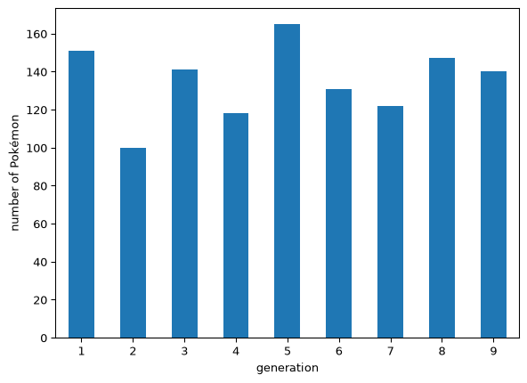
df.hist(
    column="total",
    by="generation",
    bins=np.arange(150, 1200, 50),   # the same bins for every generation
    sharex=True,
    sharey=True,
    figsize=(9, 7),
)
plt.suptitle("Distribution of total stats, per generation")
plt.show()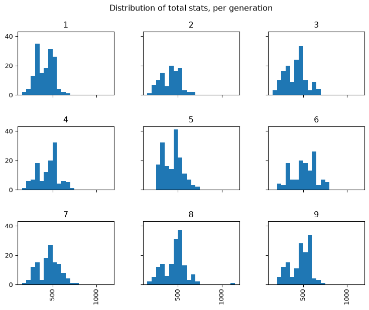
The second plot is an example of small multiples: the same chart repeated for every group, with the same axes and the same bins, so you can compare at a glance. See the user guide on visualisation for more.
A word about Polars
Polars is the main modern alternative to pandas. It is written in Rust, stores its data in the Apache Arrow format, uses all your processor cores, and can optimise a whole chain of operations before running it (its “lazy” mode). It reached version 2.0 in October 2026.
Most interesting for us: Polars has no index at all. That is a deliberate design choice, and after this lecture you can probably guess why. Rows are selected with expressions on the columns instead:
import polars as pl

pokemon = pl.read_csv(POKEMON_URL)
pokemon.filter(pl.col("HP") == 80).group_by("Type1").agg(pl.col("Total").mean())
Pandas is not going anywhere, and you will meet it in nearly every codebase that touches data. But for new projects Polars is well worth a look; see also the lecture on third party libraries.
Matplotlib
Matplotlib is the classic plotting library for Python, and once again a very large subject. We will only cover the basics, so that you know your way around. Have a look at the gallery for an idea of what is possible:
- https://matplotlib.org/stable/gallery/showcase/index.html
- https://matplotlib.org/stable/gallery/index.html
and also at the gallery of seaborn, a library built on top of Matplotlib that makes statistical plots easy.
Two interfaces
There are two ways to use Matplotlib: the pyplot interface, and the object-oriented interface. Both start with the same import, which again is a fixed convention:
import matplotlib.pyplot as pltThe pyplot interface
Pyplot is the easiest for beginners. It is state-based: Matplotlib keeps track of a “current” figure and a “current” plot area, and every function you call works on those. This way of working was copied from MATLAB.
Let’s plot the distance travelled by a falling object, d = \frac{1}{2} g t^2:
t = np.arange(0.0, 10.0, 0.2)   # seconds
g = 9.8                          # m/s²
velocity = g * t
distance = 0.5 * g * t**2plt.figure(figsize=(8, 4)) # creates a figure; it is now the "current" one
plt.plot(t, distance, "o-") # these all act on the current figure
plt.xlabel("time (s)")
plt.ylabel("distance (m)")
plt.title("Free fall")
plt.grid(True, alpha=0.3)
plt.show()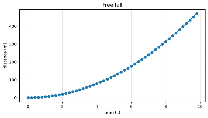
The string "o-" is a shorthand for the style: o for round markers, - for a solid line. You can add a colour too, for instance "ro--" for red markers with a dashed line.
Behind the scenes, there really are objects for the figure and the plot area. You can ask pyplot for the current ones with plt.gcf() (“get current figure”) and plt.gca() (“get current axes”).
You can put several plots in one figure with plt.subplot(rows, columns, number), which makes a new plot area “current”:
plt.figure(figsize=(8, 3))
plt.subplot(1, 2, 1)
plt.plot(t, distance)
plt.title("distance (m)")
plt.subplot(1, 2, 2)
plt.plot(t, velocity)
plt.title("velocity (m/s)")
plt.show()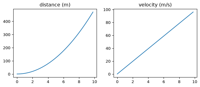
This works, but you can see how it becomes hard to follow: what any line does depends on which lines came before it.
The object-oriented interface
The alternative is to create the figure and the plot areas explicitly, and call methods on them. The function plt.subplots creates both in one go:
fig, ax = plt.subplots(figsize=(8, 4))
ax.plot(t, distance, "o-")
ax.set_xlabel("time (s)")
ax.set_ylabel("distance (m)")
ax.set_title("Free fall")
ax.grid(True, alpha=0.3)
plt.show()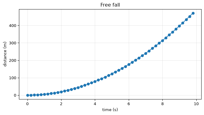
Note that the method names are slightly different: plt.xlabel(...) becomes ax.set_xlabel(...).
A word on terminology, because it is confusing. A Figure is the whole image. An Axes is one plot area inside it, with its own coordinate system. An Axis is one of the axes of that coordinate system (x or y). So a figure has one or more Axes, and each Axes has two Axis objects. The anatomy of a figure shows all the parts and their names.
With more than one plot area, plt.subplots returns them as a NumPy array:
fig, axes = plt.subplots(nrows=2, ncols=2, figsize=(8, 6))
axes[0, 0].plot(t, distance)
axes[0, 0].set_title("distance")
axes[0, 1].plot(t, velocity)
axes[0, 1].set_title("velocity")
axes[1, 0].plot(distance, velocity)
axes[1, 0].set_title("velocity vs distance")
axes[1, 1].set_title("nothing here yet")
fig.tight_layout()   # avoid overlapping labels
plt.show()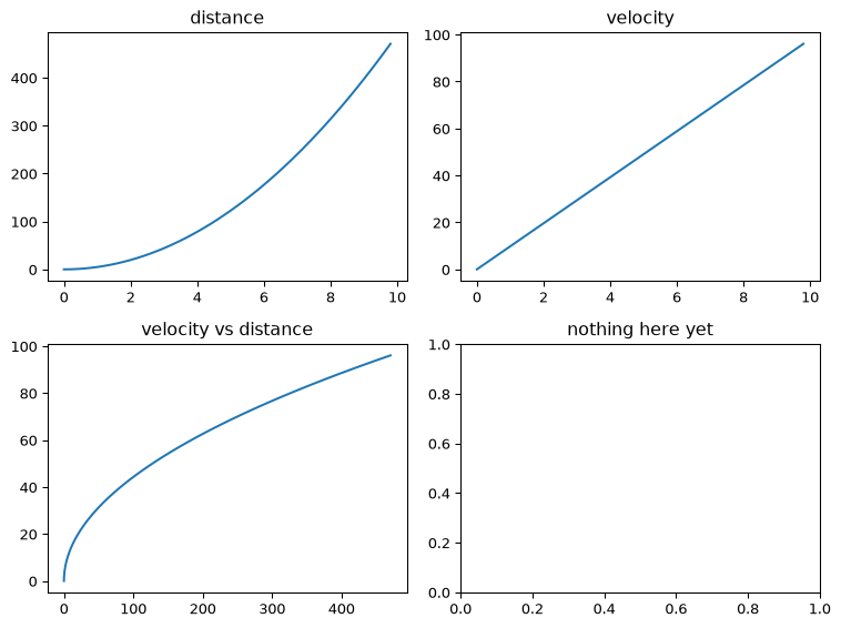
I recommend the object-oriented interface for anything beyond a quick look at your data: it is always clear which plot you are working on, and it combines well with functions. A function that draws something can take an ax argument, and the caller decides where the drawing goes.
For more complex layouts, have a look at plt.subplot_mosaic, and for complete manual control, at fig.add_axes.
Two y-axes?
What if you want distance and velocity in one plot? They have different units, so they need different y-axes. Matplotlib can do that with ax.twinx(), which adds a second y-axis on the right, but I advise against it. The two scales are independent, so where the two lines cross, or how steep one looks compared to the other, is entirely determined by the arbitrary choice of scales. Readers will see patterns that aren’t in the data.
The honest alternative is two plots stacked on top of each other, sharing the x-axis:
fig, (ax_top, ax_bottom) = plt.subplots(nrows=2, sharex=True, figsize=(8, 5))
ax_top.plot(t, distance)
ax_top.set_ylabel("distance (m)")
ax_bottom.plot(t, velocity)
ax_bottom.set_ylabel("velocity (m/s)")
ax_bottom.set_xlabel("time (s)")
plt.show()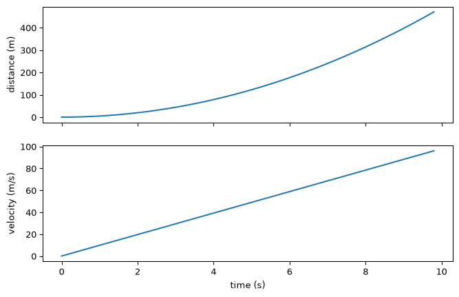
Saving figures
To save a figure to a file, use fig.savefig. The format follows from the extension: .png for an image, .svg or .pdf for vector graphics that stay sharp at any size.
fig.savefig("free_fall.png", dpi=200)
fig.savefig("free_fall.svg")
Backends: where does the figure go?
Matplotlib can draw on many kinds of “canvas”: a PNG file, a window on your screen, a web page. This is the backend, and you can see which one is active:
import matplotlib as mpl

mpl.rcParams["backend"]- In Jupyter, the default backend draws the figure as a static image below each cell. Every cell starts with a fresh figure, so make sure each plot is created within a single cell. With the magic command
%matplotlib qtyou can switch to interactive windows instead, in which you can zoom and pan. - In an ordinary Python script,
plt.show()opens a window and waits until you close it. Just likemainloop()in tkinter, it hands control over to the window until it is closed.
See the documentation on backends for details.
Matplotlib and pandas together
Pandas’ plotting functions accept an ax= argument, so you can draw into an Axes that you made yourself, and mix pandas plots with plain Matplotlib. And of course you can always hand pandas columns to Matplotlib directly.
Here is a scatter plot of attack against defense. Rather than giving each of the 18 types its own colour, which nobody could tell apart, we highlight one type and show the rest in grey:
dragons = df.loc[df["type1"] == "Dragon"]
others = df.loc[df["type1"] != "Dragon"]

fig, ax = plt.subplots(figsize=(7, 5))
ax.scatter(others["attack"], others["defense"], s=10, color="#c3c2b7", label="other types")
ax.scatter(dragons["attack"], dragons["defense"], s=20, color="#2a78d6", label="Dragon")
ax.set_xlabel("attack")
ax.set_ylabel("defense")
ax.set_title("Dragon types tend to have a high attack")
ax.legend()
plt.show()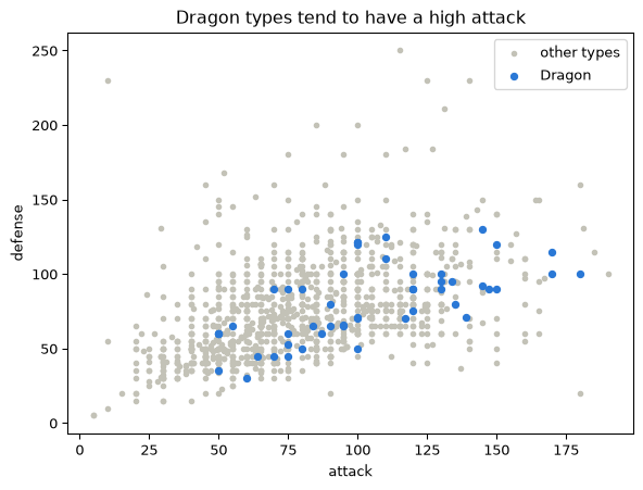
Additional resources
- 10 minutes to pandas
- pandas: indexing and selecting data
- pandas: working with missing data
- pandas: Copy-on-Write
- What’s new in pandas 3.0
- Matplotlib quick start guide
- Matplotlib cheatsheets
- Polars user guide