import numpy as npNumPy and SciPy
How Newton did it
The scientific stack
Python is enormously popular for “scientific” work: data analysis, statistics, engineering, machine learning, … That is a little ironic, because Python itself is a slow language for number crunching. The secret is a small number of third party libraries that do the heavy lifting for it:
- NumPy: arrays of numbers, and fast mathematics on them. Everything else builds on this.
- SciPy: algorithms. Optimisation, integration, statistics, signal processing, …
- pandas: tables of data. See the next lecture.
- Matplotlib: plots. Also in the next lecture.
Together with libraries built on top of them (scikit-learn, statsmodels, seaborn, …) this is often called the scientific stack or the PyData stack. Even libraries that are not built on NumPy, such as PyTorch, deliberately copy its interface, so what you learn today carries over.
To run the code in this lecture you need these packages installed in your environment, e.g.:
uv add numpy scipy matplotlibBy universal convention, NumPy is imported as np. Please don’t invent your own abbreviation: every tutorial, every Stack Overflow answer and every colleague will assume np.
NumPy arrays
NumPy was first and foremost designed for linear algebra, which is a fancy way of saying calculations with vectors and matrices. In NumPy both are called arrays:
- A vector has a length. Its
shapeattribute is(n,) - A matrix has a length and a width. Its
shapeattribute is(n, m)
vec = np.array([1, 2, 3])
vec.shape(3,)mat = np.array([[1, 2], [3, 4]])
matarray([[1, 2],
[3, 4]])mat.shape(2, 2)NumPy can also work with arrays of higher rank, sometimes called tensors:
tensor = np.array([[[1, 2], [3, 4]], [[10, 20], [30, 40]]])
tensor
array([[[ 1, 2],
[ 3, 4]],
[[10, 20],
[30, 40]]])tensor.shape(2, 2, 2)The number of dimensions is .ndim, and the total number of elements is .size:
print(vec.ndim, mat.ndim, tensor.ndim)
print(vec.size, mat.size, tensor.size)
1 2 3
3 4 8The dtype
Unlike a list, a NumPy array does not hold arbitrary objects. Every element of an array has the same type, and that type is stored once, in the dtype (data type) attribute:
int64is an integer of 64 bits (8 bytes)float64is a floating point number of 64 bits (8 bytes)- and there are many more:
int8,int16,int32,uint8,float32,bool,complex128, …
NumPy picks a suitable dtype for you, unless you tell it explicitly. A single float is enough to turn the whole array into floats:
print(np.array([1, 2, 3]).dtype)
print(np.array([1, 2, 3.0]).dtype)
print(np.array([1, 2, 3], dtype=np.int8).dtype)
int64
float64
int8Very important: the numbers inside these arrays are not the ordinary int and float objects you know from Python! They have been converted to a corresponding NumPy type:
int_vec = np.array([1, 2, 3])
int_vec[0], type(int_vec[0])
(np.int64(1), numpy.int64)float_vec = np.array([1.0, 2.0, 3.0])
float_vec[0], type(float_vec[0])(np.float64(1.0), numpy.float64)Once the dtype of an array is fixed, NumPy will not change it anymore. Instead, every new value you put into the array is converted to that dtype, whether that makes sense or not:
arr = np.array([1, 2, 3])  # dtype is int64
arr[0] = 100.7             # converted to an int64 before it is stored
arr
array([100, 2, 3])The .7 is just gone. No error, no warning. Strings suffer the same fate: a string array has a maximum length baked into its dtype (<U5 means “unicode strings of at most 5 characters”):
fruit = np.array(["apple", "kiwi"])
print(fruit.dtype)
fruit[1] = "watermelon"
fruit<U5array(['apple', 'water'], dtype='<U5')So why on earth would anyone want this? Two reasons: memory and speed.
Why NumPy? Memory
A Python list does not contain your numbers. It contains pointers (references) to Python objects, and each of those objects lives somewhere else in memory. A Python int is a full-blown object with a type, a reference count and a value, and it takes at least 28 bytes on a 64 bit machine:
import sys

sys.getsizeof(1), sys.getsizeof(10_000_000_000), sys.getsizeof(10**21)
(28, 32, 36)The list itself takes 56 bytes, plus 8 bytes for every pointer:
python_list = [1] * 100
sys.getsizeof(python_list), 56 + 8 * len(python_list)
(856, 856)Note that this number does not even include the integer objects themselves: getsizeof only counts the list and its pointers.1
A NumPy array, on the other hand, stores the raw numbers themselves, side by side in one contiguous block of memory. An int32 takes exactly 4 bytes:
numpy_arr = np.array([10] * 100, dtype=np.int32)
print(numpy_arr.itemsize, numpy_arr.nbytes)
sys.getsizeof(numpy_arr), 112 + 4 * len(numpy_arr)
4 400(512, 512)In a picture:
Python list [1, 2, 3]                       NumPy array([1, 2, 3])

 list object                                 ndarray object
┌────────────────┐                          ┌──────────────────┐
│ header         │                          │ header, shape,   │
│ (56 bytes)     │                          │ dtype=int64, ... │
├────────────────┤                          │ data pointer ────┼──┐
│ pointer ───────┼──► int object (28 bytes) └──────────────────┘  │
│ pointer ───────┼──► int object (28 bytes)                       ▼
│ pointer ───────┼──► int object (28 bytes)  ┌────────┬────────┬────────┐
└────────────────┘                           │   1    │   2    │   3    │
                                             └────────┴────────┴────────┘
                                               8 bytes each, side by side
For a handful of numbers, who cares. But this adds up quickly: a list of 30 million integers takes over a gigabyte of memory.
n = 30_000_000
(28 * n + 56 + 8 * n) / 1024**3 # in GB1.005828432738781We can check this for real with psutil, which we will meet again in the lectures on processes and threads. We will not run this code as part of these notes, since it deliberately eats a gigabyte of memory, but try it yourself:
import os

import psutil

process = psutil.Process(os.getpid())

def print_memory():
    print(f"Memory used: {process.memory_info().rss / 1024**3:.2f} GB")

print_memory()
numbers = list(range(30_000_000))
print_memory()
On my laptop this prints:
Memory used: 0.02 GB
Memory used: 1.14 GB
Restart Python and do the same with NumPy:
print_memory()
numbers = np.arange(30_000_000)  # the NumPy version of range, more on it below
print_memory()
Memory used: 0.03 GB
Memory used: 0.25 GBThat is 30 million times 8 bytes, and not a byte more. With dtype=np.int32 it would be half of that again.
Tip
If you only need a one-dimensional array of numbers and nothing else, the standard library has a little-known module array that stores the numbers compactly too. It has none of NumPy’s mathematics, but it is always available.
Why NumPy? Speed
The same design also makes NumPy much faster. Let’s add two sequences of a million numbers, once with lists and once with arrays. (Again we don’t run timing code while building these notes; your numbers will be different, but the ratio will be similar.)
import time

py_list1 = list(range(1_000_000))
py_list2 = [2 * x for x in py_list1]

t0 = time.perf_counter()
total = [x + y for x, y in zip(py_list1, py_list2)]
t1 = time.perf_counter()
print(f"Lists:  {(t1 - t0) * 1000:.1f} ms")

np_arr1 = np.arange(1_000_000)
np_arr2 = 2 * np.arange(1_000_000)

t0 = time.perf_counter()
total = np_arr1 + np_arr2
t1 = time.perf_counter()
print(f"NumPy:  {(t1 - t0) * 1000:.1f} ms")
Lists: 63.1 ms
NumPy: 2.1 msThirty times faster, and the code is shorter too. Where does that come from?
- No type checks per element. To compute
x + y, Python first has to find out whatxandyare, look up how to add them, and only then add them. NumPy knows from the dtype that it is addingint64toint64, so it checks once, not a million times. - No new objects. Every
x + yin the list version creates a brand newintobject of 28 bytes. NumPy just writes 8 bytes into a pre-allocated block. - The loop runs in compiled code. NumPy’s inner loops are written in C, and the contiguous memory layout lets the processor use its cache efficiently and even process several numbers in a single instruction (SIMD).
Writing your code as operations on whole arrays, instead of loops over elements, is called vectorisation. It is the skill to learn when working with NumPy.
The worst of both worlds
Looping over a NumPy array with ordinary Python is even slower than looping over a list, because NumPy has to wrap every element in a new np.int64 object for you. Measured on the same million numbers:
| time | |
|---|---|
sum(py_list) (builtin sum, list) |
6 ms |
np_arr.sum() (NumPy method) |
0.25 ms |
sum(np_arr) (builtin sum, NumPy array) |
46 ms |
Rule of thumb: if you are writing a for loop over the elements of a NumPy array, you are probably doing it wrong.
For linear algebra, NumPy relies on battle-tested libraries known as BLAS and LAPACK, written in C and Fortran and tuned for each processor. You can see which ones your NumPy uses with:
np.show_config()From the point of view of SciPy and pandas, NumPy is a backend: they build on its arrays and its compiled code, and add their own functionality on top.
The price: numbers of fixed size
All of this comes at a price. A Python int can be as large as you like, it simply grows when it needs more space:
8446744073709551616 * 10008446744073709551616000A NumPy int64 has exactly 64 bits, no more. Let’s do the same calculation in NumPy:
int_vec = np.array([1, 2, 8446744073709551616])
int_vec.dtypedtype('int64')int_vec * 1000array([ 1000, 2000, -1864712049423024128])The third number is negative! The true result does not fit into 64 bits, so the number overflows: the bits that don’t fit are thrown away and what remains is interpreted as a (negative) number. And note what is missing: an error message. On arrays, NumPy overflows silently.
Here is another example. The factorial 24! is a perfectly reasonable number:
import math

math.factorial(24)620448401733239439360000np.arange(1, 25).prod()np.int64(-7835185981329244160)Once again, a negative number, without any warning. The limits of each type are easy to look up:
np.iinfo(np.int64)iinfo(min=-9223372036854775808, max=9223372036854775807, dtype=int64)np.iinfo(np.int32)iinfo(min=-2147483648, max=2147483647, dtype=int32)int64 goes up to about 9.2 \times 10^{18}, which sounds like a lot, and for most purposes it is. But you don’t always have 64 bits. Smaller dtypes are very common in practice, because they save memory. For instance images are usually stored as uint8 (unsigned, 0 to 255) per colour channel. Brighten two pixels a little:
pixels = np.array([200, 250], dtype=np.uint8)
pixels + 10
array([210, 4], dtype=uint8)The second pixel was nearly white, and has now become nearly black.
This is not a theoretical problem:
- In December 2014 the music video Gangnam Style passed 2,147,483,647 views on YouTube, which is the maximum of a signed 32 bit integer. YouTube had to upgrade its view counter to 64 bits.
- Many systems store time as a signed 32 bit number of seconds since 1 January 1970. That counter overflows on 19 January 2038: the year 2038 problem.
- In 1996 the maiden flight of the Ariane 5 rocket self-destructed 37 seconds after launch, because a 64 bit floating point number was converted into a 16 bit integer that was too small to hold it.
np.array([2**31 - 1], dtype=np.int32) + 1array([-2147483648], dtype=int32)Interestingly, when you do a calculation with a single NumPy scalar rather than an array, NumPy does warn you:
np.int64(8446744073709551616) * 1000/tmp/ipykernel_12520/1858620209.py:1: RuntimeWarning: overflow encountered in scalar multiply
np.int64(8446744073709551616) * 1000np.int64(-1864712049423024128)But a warning is easy to miss, and with arrays you don’t even get that.
Always know your dtypes
Check the .dtype of your arrays, especially of data you did not create yourself, and choose the dtype explicitly when it matters. If your numbers can grow large, use a large enough type. And never use floats for money: work in integer cents, or use Decimal from the standard library.
When the numbers don’t fit at all
What does NumPy do when you hand it a number that does not fit in any of its integer types? That depends on how far off you are. Just a little bit too large, and you silently get floats:
np.array([2**63, 1])array([9.22337204e+18, 1.00000000e+00])Floats can represent huge numbers, but only with about 16 significant digits, so the exact value is lost. Larger still, and NumPy gives up and falls back to dtype=object:
np.array([2**80 + 1, 2**80 + 1, 2**80 + 1])array([1208925819614629174706177, 1208925819614629174706177,
1208925819614629174706177], dtype=object)An object array is just a list of pointers to ordinary Python objects again. It works, but all the memory and speed advantages are gone.
Something similar happens if you mix types that have nothing in common. NumPy will find a dtype that fits everything, and that may well be a string:
np.array([1, 2, "a"])array(['1', '2', 'a'], dtype='<U21')Floating point numbers
Floats don’t wrap around like integers do. Instead they have two other problems. First, they have limited precision. A float64 has about 16 significant digits, a float32 only about 7. So float32 cannot even represent all integers above 2^{24} = 16\,777\,216:
np.float32(16_777_217)np.float32(1.6777216e+07)Second, when a float gets too large it becomes infinity:
np.array([1e308]) * 10array([inf])Not a number
There is one more special float value you need to know about: nan, short for not a number. It is the result of undefined calculations such as 0 / 0 or inf - inf, and it is very often used to mean “missing data”.
nan is contagious: any calculation involving nan gives nan. So a single missing value spoils your whole sum:
data = np.array([1, 2, 3, np.nan])
data.sum()np.float64(nan)NumPy has variants of the usual functions that skip nan:
np.nansum(data), np.nanmean(data)(np.float64(6.0), np.float64(2.0))And nan is the only value that is not equal to itself, so you cannot test for it with ==:
print(np.nan == np.nan)
print(np.isnan(data))
False
[False False False True]Finally, and this will haunt us in the next lecture: integers have no nan. An array of integers with one missing value therefore becomes an array of floats.
np.array([1, 2, np.nan]).dtypedtype('float64')Working with arrays
Creating arrays
Apart from np.array(...) there are many functions that create arrays for you. Two important ones are np.arange and np.linspace. The first is the NumPy version of the builtin range. The second, np.linspace(x, y, n), divides the interval [x, y] into n equally spaced points, including both ends:
np.arange(1, 15, 2)array([ 1, 3, 5, 7, 9, 11, 13])np.linspace(0, 1, 5)array([0. , 0.25, 0.5 , 0.75, 1. ])np.arange accepts a float step too, but because of rounding errors you cannot always predict how many elements you will get. Is 1.3 included here?
np.arange(1, 1.3, 0.1)array([1. , 1.1, 1.2, 1.3])It is, sort of. As a rule, use arange for integers and linspace for floats.
Some more:
np.zeros(3), np.ones((2, 3)), np.full(3, 7.5)(array([0., 0., 0.]),
array([[1., 1., 1.],
[1., 1., 1.]]),
array([7.5, 7.5, 7.5]))np.eye(3) # identity matrixarray([[1., 0., 0.],
[0., 1., 0.],
[0., 0., 1.]]).reshape gives you the same numbers in a different shape:
np.arange(12).reshape(3, 4)array([[ 0, 1, 2, 3],
[ 4, 5, 6, 7],
[ 8, 9, 10, 11]])For random numbers, create a random generator first, and get your numbers from there. Giving it a seed makes the results reproducible:
rng = np.random.default_rng(seed=42)
rng.integers(1, 7, size=10)  # ten dice
array([1, 5, 4, 3, 3, 6, 1, 5, 2, 1])rng.normal(loc=0, scale=1, size=3)array([-1.30217951, 0.1278404 , -0.31624259])
Note
In older code you will see np.random.seed(42) followed by np.random.rand() and friends. That is the legacy interface, which uses one hidden global random state shared by all your code. The default_rng style is the recommended one: every generator has its own state, so different parts of your program don’t influence each other’s random numbers.
Calculating with arrays
Arithmetic on arrays works element by element:
a = np.array([1, 2, 3, 4])
b = np.array([10, 20, 30, 40])

print(a + b)
print(a * b)
print(a ** 2)
print(b / a)
print(b // 3)
[11 22 33 44]
[ 10 40 90 160]
[ 1 4 9 16]
[10. 10. 10. 10.]
[ 3 6 10 13]So do comparisons, which give an array of booleans:
a > 2array([False, False, True, True])And all the mathematical functions you know from the math module have a vectorised counterpart, the so-called universal functions or ufuncs:
np.sqrt(a), np.exp(a), np.sin(a)(array([1. , 1.41421356, 1.73205081, 2. ]),
array([ 2.71828183, 7.3890561 , 20.08553692, 54.59815003]),
array([ 0.84147098, 0.90929743, 0.14112001, -0.7568025 ]))Arrays also have methods to summarise them, the aggregations:
print(a.sum(), a.mean(), a.std(), a.min(), a.max(), a.argmax())10 2.5 1.118033988749895 1 4 3For arrays with more than one dimension, you can choose along which axis to aggregate. axis=0 collapses the rows (so you get one result per column) and axis=1 collapses the columns (one result per row):
m = np.arange(12).reshape(3, 4)
m
array([[ 0, 1, 2, 3],
[ 4, 5, 6, 7],
[ 8, 9, 10, 11]])print(m.sum()) # everything
print(m.sum(axis=0)) # one number per column
print(m.sum(axis=1)) # one number per row66
[12 15 18 21]
[ 6 22 38]The same axis argument comes back in pandas, so make sure this clicks.
Indexing and slicing
For a one-dimensional array, indexing and slicing work just like with lists:
v = np.arange(10, 20)
v[0], v[-1], v[2:5], v[::3]
(np.int64(10), np.int64(19), array([12, 13, 14]), array([10, 13, 16, 19]))For a two-dimensional array, you put both indices inside one pair of brackets, separated by a comma. A : means “everything along this axis”:
m = np.arange(12).reshape(3, 4)
print(m[1, 2])     # row 1, column 2
print(m[1])        # row 1
print(m[:, 2])     # column 2
print(m[1:, :2])   # rows 1 and onwards, columns 0 and 1
6
[4 5 6 7]
[ 2 6 10]
[[4 5]
[8 9]]You can also index with a list of positions, this is called fancy indexing:
v[[0, 2, 4]]array([10, 12, 14])Or, most usefully, with an array of booleans of the same length. You get exactly those elements where the mask is True:
mask = v % 2 == 0
print(mask)
print(v[mask])
[ True False True False True False True False True False]
[10 12 14 16 18]Usually you write this in one go:
v[v % 2 == 0]array([10, 12, 14, 16, 18])To combine conditions you need the operators & (and), | (or) and ~ (not). The keywords and, or and not don’t work, because they want to turn the entire array into a single True or False, and NumPy refuses to guess what you mean by that:
v[(v > 12) and (v < 17)]--------------------------------------------------------------------------- ValueError Traceback (most recent call last) Cell In[55], line 1 ----> 1 v[(v > 12) and (v < 17)] ValueError: The truth value of an array with more than one element is ambiguous. Use a.any() or a.all()
v[(v > 12) & (v < 17)]array([13, 14, 15, 16])Mind the parentheses: & binds more strongly than >, so without them v > 12 & v < 17 means something completely different. All of this works exactly the same in pandas, so you will be using it a lot.
Views and copies
Here is something that surprises people coming from lists. Slicing a list makes a copy. Slicing a NumPy array does not: you get a view, a new array object that looks at the same memory. Modify the view, and you modify the original:
original = np.arange(10)
view = original[2:5]
view[0] = 100
original
array([ 0, 1, 100, 3, 4, 5, 6, 7, 8, 9])NumPy does this for performance: you don’t want to copy a gigabyte of data just to look at a part of it. But it means a function that receives a slice of your data can modify your data. If you need an independent copy, ask for one:
original = np.arange(10)
independent = original[2:5].copy()
independent[0] = 100
original
array([0, 1, 2, 3, 4, 5, 6, 7, 8, 9])Fancy indexing and boolean masks always give you a copy, because the selected elements are in general not next to each other in memory. np.shares_memory tells you which is which:
original = np.arange(10)
print(np.shares_memory(original, original[2:5]))
print(np.shares_memory(original, original[[2, 3, 4]]))
print(np.shares_memory(original, original[original > 4]))
True
False
FalseBroadcasting
What happens if you combine arrays of different shapes? The simplest case you have already seen: an array and a single number. The number is used for every element:
np.array([1, 2, 3]) * 10array([10, 20, 30])NumPy generalises this idea, and calls it broadcasting. If one array has length 1 along some axis, it is stretched along that axis to match the other one. A column of shape (3, 1) times a row of shape (4,) gives a whole table of shape (3, 4):
column = np.arange(1, 4).reshape(3, 1)
row = np.arange(1, 5)
column * row
array([[ 1, 2, 3, 4],
[ 2, 4, 6, 8],
[ 3, 6, 9, 12]])This is a very compact way to compute “every combination” without writing any loops. If the shapes can’t be matched, you get an error:
np.arange(3) + np.arange(4)--------------------------------------------------------------------------- ValueError Traceback (most recent call last) Cell In[62], line 1 ----> 1 np.arange(3) + np.arange(4) ValueError: operands could not be broadcast together with shapes (3,) (4,)
The full rules are in the documentation. When in doubt, print the .shape of everything involved.
Linear algebra
Since arithmetic works element by element, * is not the matrix product you know from linear algebra. For that, Python has had a dedicated operator @ since version 3.5 (PEP 465), and NumPy was the reason it was added:
m = np.array([[1, 2], [3, 4]])
print(m * m)   # element by element
print(m @ m)   # matrix product
print(m.T)     # transpose
[[ 1 4]
[ 9 16]]
[[ 7 10]
[15 22]]
[[1 3]
[2 4]]The submodule np.linalg contains the usual suspects: determinants, eigenvalues, inverses, and solving systems of linear equations. For instance, to solve
\begin{aligned} 2x + y &= 3 \\ x + 3y &= 5 \end{aligned}
A = np.array([[2.0, 1.0], [1.0, 3.0]])
b = np.array([3.0, 5.0])
np.linalg.solve(A, b)
array([0.8, 1.4])(Use solve rather than computing the inverse with np.linalg.inv and multiplying: it is both faster and more accurate.)
NumPy 2: reading older code
NumPy 2.0 was released in June 2024, and it changed a number of things. Lots of code on the internet (and a lot of what AI assistants have learned from) predates it, so here is what to look out for:
- On Windows, the default integer type used to be
int32. If you see# dtype is int32in an older notebook, that is why. It is nowint64everywhere. - Scalars are now printed with their type,
np.float64(1.0)rather than1.0. - A number of aliases were removed:
np.float_,np.NaN,np.Inf, … Usenp.float64,np.nan,np.inf. The error message tells you what to use instead. - The rules for mixing NumPy and Python numbers changed (NEP 50). A Python number now adapts to the NumPy type rather than the other way around, so
np.float32(3) + 3.0stays afloat32, andnp.int8(100) + 200raises anOverflowErrorbecause 200 does not fit in anint8. np.array(x, copy=False)used to mean “avoid a copy if you can”; it now means “never copy”, and raises an error if a copy is needed. Usenp.asarray(x)for the old behaviour.
The migration guide has the complete list.
SciPy: how Newton did it
SciPy is a large collection of scientific algorithms built on top of NumPy. Most of it belongs in a specialised course on numerical methods or statistics, so we will only look at one example in depth, and then take a quick tour.
The problem
Here is an innocent-looking equation:
\cos(x) = x
There is no formula that gives you the solution. But a plot tells us there is exactly one, somewhere around x = 0.75. (Don’t worry about the details of plotting yet, that is for next lecture.)
import matplotlib.pyplot as plt

x = np.linspace(0, np.pi / 2, 200)
plt.plot(x, np.cos(x), label="cos(x)")
plt.plot(x, x, label="x")
plt.xlabel("x")
plt.legend()
plt.grid(True, alpha=0.3)
plt.show()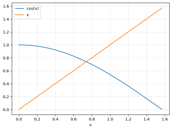
To find the solution, we rewrite the equation as f(x) = 0 with f(x) = \cos(x) - x, and go looking for a root of f.
Newton’s method
Isaac Newton described a method for this around 1669, for polynomials, and Joseph Raphson published a simpler version in 1690; it is known as the Newton-Raphson method. The idea is simple: start with a guess x_0. Near x_0, the function looks a lot like its tangent line, and it is easy to see where that tangent line crosses zero. Take that as your next guess, and repeat:
x_{n+1} = x_n - \frac{f(x_n)}{f'(x_n)}
For our function the derivative is f'(x) = -\sin(x) - 1. In Python:
def f(x):
    return np.cos(x) - x

def f_prime(x):
    return -np.sin(x) - 1

x = 1.0
for i in range(5):
    x = x - f(x) / f_prime(x)
    print(i, x)
0 0.7503638678402439
1 0.7391128909113617
2 0.739085133385284
3 0.7390851332151607
4 0.7390851332151607Look at how fast that converges: the number of correct digits roughly doubles with every step. After four steps we have the answer to the full precision of a float64.
Because f and f_prime are written with NumPy functions, the very same code also works on an array. We can run Newton’s method from many starting points at once, without changing a single line:
x = np.array([-1.55, -1.0, 0.0, 1.0, 2.0])
for i in range(8):
    x = x - f(x) / f_prime(x)
x
array([344.86926785, 0.73908513, 0.73908513, 0.73908513,
0.73908513])All but one of them have found the solution. The one that started at -1.55 is lost: at x = -\pi/2 \approx -1.571 the derivative is zero, so the tangent line is horizontal, and nearby the tangent line sends you very far away. Newton’s method is fast, but it needs a reasonable starting point.
scipy.optimize
Of course you don’t have to write this yourself. The submodule scipy.optimize has a whole range of root finders, including Newton’s own:
from scipy import optimize

optimize.newton(f, x0=1.0, fprime=f_prime)np.float64(0.7390851332151607)If you don’t know the derivative, leave out fprime, and SciPy uses the secant method instead, which approximates the derivative from the previous steps.
The more general function is optimize.root, which can also solve systems of several equations in several unknowns:
result = optimize.root(f, x0=0)
result
message: The solution converged.
success: True
status: 1
fun: [ 0.000e+00]
x: [ 7.391e-01]
method: hybr
nfev: 11
fjac: [[-1.000e+00]]
r: [ 1.674e+00]
qtf: [-2.668e-13]The result is an OptimizeResult. That is a dict that also allows attribute access, much like the AttributeDict we built in OOP III:
print(isinstance(result, dict))
print(result.x, result["x"])
print(result.success, result.nfev)
True
[0.73908513] [0.73908513]
True 11Always check .success. Numerical algorithms can fail, and they will happily hand you a result anyway.
If you know an interval where f changes sign, optimize.root_scalar with a bracket uses a method that is slower than Newton’s but guaranteed to converge:
optimize.root_scalar(f, bracket=[0, 1]).root0.7390851332151559A quick tour of the rest
SciPy has a lot more to offer. A small sample:
Integration with scipy.integrate. For instance \int_{-\infty}^{\infty} e^{-x^2} dx = \sqrt{\pi}:
from scipy import integrate

value, error_estimate = integrate.quad(lambda x: np.exp(-x**2), -np.inf, np.inf)
value, np.sqrt(np.pi)
(1.7724538509055159, np.float64(1.7724538509055159))Statistics with scipy.stats: probability distributions, random variables, hypothesis tests, … For instance, if heights are normally distributed with mean 170 cm and standard deviation 10 cm, what fraction of people is shorter than 190 cm?
from scipy import stats

stats.norm(loc=170, scale=10).cdf(190)np.float64(0.9772498680518208)Or a t-test, to check whether two samples plausibly come from distributions with the same mean:
rng = np.random.default_rng(seed=42)
sample_a = rng.normal(loc=0.0, size=50)
sample_b = rng.normal(loc=0.5, size=50)
stats.ttest_ind(sample_a, sample_b)
TtestResult(statistic=np.float64(-1.4140514070147219), pvalue=np.float64(0.1605158425424986), df=np.float64(98.0))And then there is scipy.interpolate, scipy.linalg, scipy.signal, scipy.fft, scipy.sparse, scipy.spatial, … Browse the documentation to get an idea, so that you know where to look when you need it.
Demo: Newton’s fractal
To finish, let’s push Newton’s method a little further, and let NumPy show off. The equation z^3 = 1 has only one real solution, z = 1, but in the complex numbers it has three:
1, \quad e^{2\pi i/3}, \quad e^{-2\pi i/3}
Newton’s method works for complex numbers too. So for each starting point in the complex plane, we can ask: which of the three solutions does it end up at?
NumPy has a complex dtype, and Python writes the imaginary unit as 1j. We build a grid of 500 × 500 starting points with broadcasting, and then run Newton’s method on all 250 000 of them simultaneously:
n = 500
re = np.linspace(-1.5, 1.5, n)
im = np.linspace(-1.5, 1.5, n)
z = re[np.newaxis, :] + 1j * im[:, np.newaxis]   # shape (n, n), dtype complex128

for _ in range(40):
    z = z - (z**3 - 1) / (3 * z**2)

roots = np.array([1, np.exp(2j * np.pi / 3), np.exp(-2j * np.pi / 3)])
# distance from every point to every root: shape (n, n, 3)
distances = np.abs(z[:, :, np.newaxis] - roots)
closest = distances.argmin(axis=2)               # 0, 1 or 2 for every point
Colour every starting point according to the solution it converged to:
from matplotlib.colors import ListedColormap

fig, ax = plt.subplots(figsize=(6, 6))
ax.imshow(
    closest,
    extent=(-1.5, 1.5, -1.5, 1.5),
    origin="lower",
    cmap=ListedColormap(["#2a78d6", "#eb6834", "#1baf7a"]),
)
ax.plot(roots.real, roots.imag, "w+", markersize=12, markeredgewidth=2)
ax.set_xlabel("real part")
ax.set_ylabel("imaginary part")
ax.set_title("Which root does Newton's method find for $z^3 = 1$?")
plt.show()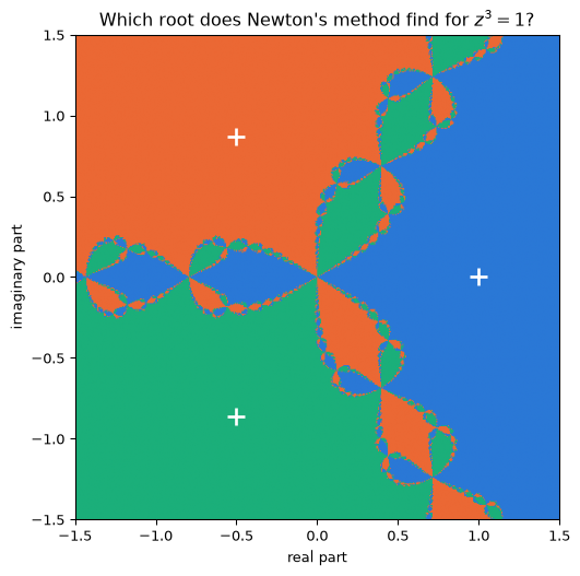
Near each solution, the answer is what you would expect. But in between, the three basins interleave in an infinitely detailed pattern: a fractal. Small changes in the starting point lead to completely different answers, which is exactly the “lost” starting point we saw earlier, in two dimensions.
Additional resources
- NumPy: the absolute basics for beginners
- From Python to NumPy, a free book by Nicolas Rougier on vectorisation
- NumPy 2.0 migration guide
- SciPy User Guide
- Building SciPy with Flang, on the Fortran that is still hiding inside SciPy, and what it takes to compile it on Windows
Footnotes
In this particular example all 100 pointers point to the same object
1, because CPython keeps the small integers from -5 to 256 around as singletons. A list of 100 different large numbers needs 100 separate integer objects.↩︎